Dead Weight Testers | Master Test Gauges | Pressure Calibrators | Temperature Calibrators | Multifunction Calibrators | Electrical Test Equipment | Decade Boxes | Pressure Gauges | Instrument Valves | DBB & Monoflanges | Mixers

Budenberg Middle East Trading LLC,  Office no. 217  Bil Obaida Building,  Al Nahda Road,  Al Qusais 1,  Dubai,  United Arab Emirates

Pressure is defined as “Force per Unit Area”.

In other words, Pressure (P) = Force (F) / Area (A) = (mass) m x (Gravity) g / Area (A)

Its Magnitude depends on the Force of Impact over a defined Area.

Let us understand it in a simple layman’s language:

MASS is a measure of the “bulk” of an object. A 1 kilo sand bag has the same mass whether it is on earth or in outer space. However, the FORCE (F) it exerts on a bench top, its WEIGHT, is due to the action of GRAVITY (g). In outer space, it still has mass, but no weight.

Gravity works like an acceleration. Let go of the sand bag, and it accelerates rapidly towards the ground. All the time it is on the bench, it is held up by a force equal to its mass times the gravitational acceleration.

The acceleration due to gravity has been measured at around 9.80665 m/sec².

So if a Force (F) of 1 kilogram accelerates a mass (m) of 1 kilogram at 1 m/s².  We call this 1 Newton Force.

If we now spread the Force of one Newton over a standard area of one square metre, we get 1 N/m² Pressure and call it a Pascal (Pa for short).

This is a pretty small pressure, but we can always multiply it up to

       1 kilopascal (kPa) = 1000 pascals  (10³ Pa) 

  1 Megapascal (MPa) = 1 000 000 pascals (10Pa)

                                    1 bar = 1 00 000 pascals (105 Pa)

The air we breathe at sea level has a pressure of around 101 325 pascals, scientists and engineers call this a bar. For small values this is divided into 1000 millibars (mbar).

The Pascal and its multiples are the internationally used units of pressure in which everyone is supposed to work.

These units are Bar, Psi, kPa, Mpa, Kg/cm², in Water, mm Water, Hg Water etc.  

The measurement of  Zero Pressure at Atmospheric Pressure is known as Gauge Pressure.

The Instrument which is designed to measure Pressure values with reference to Atmospheric Pressure and indicates ZERO is said to measure Gauge Pressure.

So, Zero Gauge Pressure is equal to 1000 mbar Atmospheric Pressure

It is Commonly taken to mean pressures below, and often considerably below, Atmosphere and does not have separate Units. It is also known as Negative Gauge Pressure

We don’t say “Vacuum is Force per Unit Area”. 

A system with no Molecules is said to have Zero Pressure or Vacuum (-1000 mbar / -30” Hg / -760 mmHg)

Pressure Measured on a Scale which uses Zero Pressure (Vacuum) as its reference is known as Absolute Pressure. Absolute Pressure compares the measured value with a full vacuum and is therefore, at the earth’s surface, numerically around 1 bar greater than the Gauge Pressure. 

This means 1000 mbar Absolute Pressure = Zero Gauge Pressure

We can also say, the sum of Gauge Pressure and Atmospheric Pressure is Absolute Pressure.

In outer space, there is no atmosphere, so gauge and absolute are synonymous

The Pressure Difference between two systems is known as Differential Pressure. In a Differential Pressure, the reference Pressure may be either Zero or Atmospheric Pressure or some other value.

With Differential Pressure, the user provides both the measured pressure and the reference pressure. The advantage is that, small differences between two high pressures may be measured accurately. 

For Example: Flow of Gas along a Pipeline depends on Pressure Difference between the ends of the Pipe and in practice both ends are usually at High Pressure.

The Atmospheric Pressure is the Force exerted on a unit surface Area caused by earth’s Gravitational attraction of  the air vertically above that Area.

Atmospheric Pressure Decreases with Increasing Altitude.

Atmospheric Pressure at surface of the earth varies between about 970 mbar and 1030 mbar.

If you drop a 1 kilo weight at a point on the earth where the gravity is exactly “standard”, then it will accelerate as it falls at 9.80665 m / s² because it has a gravitational force of 1 kilo acting on it. The Newton is the force that accelerates a 1 kilo mass by 1 m / s² and is therefore 1/9.80665 of a kilo. 

Firstly, “lbf/in²” is the more precise term, as it stands for pounds-force per square inch, but psi is what everyone has been calling it for years.

Note that I underlined force. It is important to distinguish between mass, which is the quantity of substance, force which is an amount of push or pull and weight which is the special force we feel when gravity acts upon a mass.

While “psi” does not contain the initial of the magic word “force”, it’s very handy for those who like to write psig (for gauge), psia (for absolute) and even psid (for differential). So it’s OK to use this vernacular abbreviation.

The 1/2”API connection which to all intents and purposes is identical specifies a rating of 10000 psi (690 bar). There is sadly no clear indication whether this is an actual or a nominal rating. One thing is certain. However, the joint does have a pretty good safety factor (at room temperature) and plenty of users have instruments in service up to 1000 bar (14500 psi). Our policy is always to recommend the HP cone joint (Code “V”) for pressures over 10000 psi / 600 bar instrument ranges. If customers really want to go higher than this, we should not challenge their expertise but like a user friendly PC just say “ARE YOU SURE?” and get a written confirmation before proceeding.

Bourdon Tube Gauges are calibrated at 20°C and the effect of temperature will incur an error of ± 0.4% percentage of span for every 10°C difference on rising or falling pressure. Bourdon Tube Gauges can be used on fluids up to 200°C as long as the temperature seen by the gauge is not greater than 70°C. 

Therefore at high temperatures the gauge will still operate but the readings will be totally inaccurate but the readings should return to the calibrated state once the unit has had time to cool down.

The magnitude of the applied pressure which physically destroys a device is called Burst Pressure. It is also known as rupture pressure.

There are many options like use of Syphons, Loops or impulse tubing can all be used to reduce the Temperature seen by the gauge to acceptable levels. If this is not practical then again Diaphragm Seal Gauges will have to be considered.

Usually Pressure Gauges are provided with over range protection from 115% to 200% depending upon the pressure ranges and the type of tube. If overloads greater than the overload gauge can’t withstand then Gauge Saver (overload protection valve) is required and must be installed beneath the gauge.

Vibration can be easily ascertained by touching the unit

Solutions:

  • Fit unit with a Viscous Damped Movement (VDM) or Fill case with Glycerine / Silicone Oil
  • Remote mount the gauge off the equipment

Note: If no vibration is felt then the likely source of the problem will be pressure pulsations in the line. 

Benefits of Viscous Damped Movement

  • Damping effect is applied to the mechanism at two key operational points. No loss or degradation of accuracy.
  • Easier to recalibrate with no messy fluids to remove/replace.
  • Unit weight is half that of a filled gauge
  • Increased life cycle – we guarantee a unit fitted with a damped movement for 1,000,000 cycles where the guarantee for filled gauges is only 200,000

Disadvantages of Glycerine Filled Cases

  • The action of dragging the pointer through the viscous fluids adds a load to the pointer that can result in accuracy errors.
  • Puts extra strain on the installation, particularly on small schedule pipes.
  • Fluid can leak out that could cause a Health & Safety hazard.
  • Units are very messy during recalibration whereby they have to be emptied
  • The unit weight is effectively doubled

This is probably because pressure peaks or pulsations are present in the line normally produced by a pump or solids in the medium.

Solutions:

  • Install a Pressure Snubber
  • Fit unit with a Check Screw
  • Fit a VDM or liquid fill case

If oscillations cover 10% of scale then Glycerine filling or fitting VDM is lowest cost solution.  Please be aware that filling the case with Glycerine or similar fluid will not prevent fatigue failure of the movement or sensing element. A VDM is the preferred choice.

If oscillations cover 50% of scale then the unit should be fitted with a Checkscrew and a VDM. If oscillations are over 50% then a Pressure Snubber and a VDM should be fitted.

Check-screw is fitted into the inlet of the gauge body which reduces the volume of medium passing into the instrument. The effect of this is to deaden the response time of the instrument.

Snubber can be internal or externally fitted and allows user adjustment to the required damping.  

Diaphragm or Chemical Seals are a mechanical barrier to protect delicate Instrumentation from the harsher process fluids and conditions. The principle is that the bourdon tube pressure gauge is liquid filled and installed in a sealed system. The interface between the sealed system and the pressure medium is a flexible diaphragm.

The diaphragm seals are principally for applications where a bourdon tube would become blocked, or where the pressure medium would corrode the bourdon tube materials.

Typical Applications are:

  • Clogging media – sewage, slurries, adhesives etc.
    Chemical Processes such as wet chlorine, sulphuric acid and peroxide and where the medium is at an elevated temperature but would solidify at lower temperatures (such as at the end of a bourdon tube).
  • To eliminate dead space and allow the system to be sterilized.
  • High process temperature.
  • For low pressure applications, we would offer a Schaffer diaphragm seal gauge.

Electric current is defined as the rate at which charge flows through a surface or the cross section of a wire. There are two ways to write the definition of electric current:

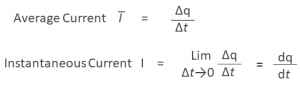
The unit of current is the ampere (A), which is named for the French scientist André-Marie Ampère (1775–1836). An ampere is a fundamental unit in the International System. Since charge is measured in coulombs and time is measured in seconds, an ampere is the same as a coulomb per second.

A difference in electric potential gives rise to an electric field. The electric field is the force per charge acting on an imaginary test charge at any location in space. The work done placing an actual charge in an electric field gives the charge electric potential energy.

A difference in electric potential gives rise to an electric field. The electric field is the force per charge acting on an imaginary test charge at any location in space. The work done placing an actual charge in an electric field gives the charge electric potential energy.

Ohm’s law states Current is directly proportional to Voltage that is


The ohm is a derived unit.

Factors affecting resistance

The resistance of the wire which is:

  • Directly proportional to the length of the wire R∝ 
  • Inversely proportional to the cross sectional area of the wire that is R α 1/A
  • Directly proportional to the resistivity of the material of the that is R α ρ

                                                               Therefore, the resistance of the wire is R = ρ / A

                                                              The unit of resistivity is the ohm meter

                                                              Therefore,  R  =  ρ / A   =   [ Ω  =  (Ωm) (m)/ (m²) ]

Points to be noted:

  1.  The resistivity of most metals increases with increasing temperature.
  2.  Resistivity is approximately directly proportional to absolute temperature for many metals over some range of temperatures.
  3.  Superconductivity is the complete and absolute loss of resistivity in some materials when cooled below a critical temperature.
  4.  Resistance is a property of objects. Resistivity is a property of materials.


The Electric Power (P) is defined as the product of the strength of the moving charges (Voltage, V) and the amount of moving charges (Current, I) power transferred by an electric current. The unity for the Power is Watt.

                                                                                                    P  =  (V) (I)

 Using Ohm’s Law, it can be expressed as:

                                                                              P  =  (IR) (I)   =   I²R   =   V² / R

The Electric Energy, E delivered by an electric current is defined as the product of its power and time over which it flows. In other words, it is the product of voltage (V), current (I) and time (t) and is expressed as:

                                                                             E   =   P.t    =    V.I.t

The unit for Energy is joules.

Using Ohm’s Law, it can be expressed as:

                                                                            E    =   I² R t   =   V²t  /  R 

From above, Electric power (P) can be calculated as energy consumption (E) divided by the time consumed (t):

                                                                            P   =   E/t     where P is in watts, E is in joules and t is in seconds

In the case of electric power consumption by homes and businesses, it is mostly sold by the kilowatt hour, which is running time in hours multiplied by the power in kilowatts. An electricity meter is used to measure the amount of power consumption.

Heat is a form of energy that flows from one place to another and is scalar quantity. The unit of energy is the joule (J). Heat is therefore measured in joules. Before this was known, however, heat had its own special units; like the calorie and the British thermal unit [Btu]. These are still widely used in for some reason — calorie for food energy (which is really a kilocalorie) and Btu for furnaces, air conditioners, stoves, and refrigerators.

We will know more about heat while explaining theoretical definition of temperature.

Theoretical definition

One has to be careful when defining temperature not to confuse it with heat. Heat is a form of energy. Temperature is something different. The hotter something is, the higher its temperature. The cooler it is, the lower is its temperature. Therefore we can say, the temperature is a measure of hotness or coldness.

Quantities in science are typically defined operationally (through the process by which they are measured) or theoretically (in terms of the theories of a specific discipline). We will begin with a theoretical definition of temperature and end with an operational definition.

To understand it theoretically, we should already know:

  1. If a system has the ability to work it possesses energy.
  2. Energy comes in two basic forms: the kinetic energy of motion and the potential energy of position.
  3. Energy is conserved. Which means it cannot be created or destroyed. When one form of energy decreases another form must increase.

The archetypal example of this is the rock at the top of a hill. Due to its height above the bottom of the hill, it possesses gravitational potential energy. Give it a push and it will start to roll. If we assume the ideal situation of a closed system where no energy is lost on the way down, then the rock’s initial potential energy will equal its final kinetic energy.

Now take the archetypal example one step further. Assume the rock crashes into a wall. Neither the rock nor the wall is elastic, so the rock comes to a halt. Now it appears as if we have violated the law of conservation of energy. The kinetic energy is lost and nothing has come along to replace it. Where has the energy gone?

The answer to this question is inside the rock. The energy has been transformed from the external energy visible as the motion of the rock as a whole to the internal energy of the motion of the invisible parts that make up the rock. The two energies are identical in size, but different in appearance. External conductors and is visible because it is organized. The translational kinetic energy of a rock is due to coordinated motion. All the parts all move forward together. The rotational energy is also coordinated. The parts all rotate together around the centre of mass. In contrast, the internal kinetic energy of a rock is invisible since the pieces are so small and numerous and their motion is completely uncoordinated. Their motions are statistically random with a mean value of zero making the energy largely invisible to us macroscopic beings.

Potential energy can also exist in external and internal forms. Internal potential energy is responsible for latent heat. If objects have internal energy, they exchange this energy. This is known as the thermal contact. The objects responsible for carrying the internal are known as atoms. These atoms in large numbers in uncoordinated motion will transfer internal energy in one direction and different times and places will run in opposite direction. This results in the net or overall transfer of internal energy. This is known as heat. If the net exchange of internal energy is zero; that is, if no heat flows from one region to another; then the whole system is said to be in thermal equilibriumHeat, then, is the net transfer of internal energy from one region to another

Two regions in thermal contact have the same temperature when there is no net exchange of internal energy between them. Temperature, then, is what determines the direction of heat flow — out of the region with the higher temperature and into the region with the lower temperature. In more concise terms, heat flows from hot to cold. That’s the theoretical definition of temperature.

Operational Definition

Temperature is measured with a thermometer. The basic operating principle behind all thermometers is that there is some quantity, called a thermometric variable that changes in response to changes in temperature. The relationship between temperature and the thermometric variable may be direct or inverse or it may be determined by a polynomial or power function. In any case, it is the thermometric variable that gets measured. There is no way to measure temperature directly.

 Types of thermometers

The units/scales for temperature are Fahrenheit, Celsius and Kelvin.

Most unit conversions are done by scaling. You take a number with a unit and multiply (or divide) by a conversion factor to get a new number with a new unit. The number by itself may be larger or smaller after the conversion, but the number with the unit is identical since the conversion factor is a ratio equal to one.  The comparison of these scales is as shown:

Thermocouple technology is based on the Seebeck effect. It is a pair of dissimilar metal wires joined at one end, which generates a net thermoelectric voltage between the open pair according to the temperature difference between the ends.

The term thermocouple refers to the complete system for producing thermal voltages and generally implies an actual assembly (i.e. a sheathed device with extension leads or terminal blocks).

In 1821 a German physicist named Thomas Johann Seebeck discovered the thermoelectric effect, which forms the basis of modern thermocouple technology. He observed that an electric current flows in a closed circuit of two dissimilar metals if their two junctions are at different temperatures. The thermoelectric voltage produced depends on the metals used and on the temperature relationship between the junctions. If the same temperature exists at the two junctions, the voltage produced at each junction cancel each other out and no current flows in the circuit. With different temperatures at each junction, different voltages are produced and current flows in the circuit. A Thermocouple can therefore only measure temperature differences between the two junctions.

The junction that is put into the process and exposed to measured temperature is called the HOT JUNCTION. The other junction which is at the last point of thermocouple material and which is almost always at some kind of measuring instrument is called the COLD JUNCTION.

The two conductors and associated measuring junction constitute a thermo-element and the individual conductors are identified as the positive or negative leg.

Thermocouples are available either as bare wire (‘bead’ thermocouples) which offer low cost and fast response times or built into probes. A wide variety of probes are available, suitable for different measuring applications (industrial, scientific, food temperature, medical research etc).

The change in material EMF with respect to a change in temperature is called the Seebeck coefficient or thermoelectric sensitivity. This coefficient is usually a nonlinear function of temperature.

A thermocouple is always formed when two metals are connected together. For example, when the Thermo element conductors are joined to copper cable or terminals, thermal voltages can be generated at the transition. In this case, the second junction can be considered as located at the connection point (assuming the two connections to be thermally common). The temperature of this connection point (terminal temperature) if known, allows computation of the temperature at the measuring junction. The thermal voltage resulting from the terminal temperature is added to the measured voltage and their sum corresponds to the thermal voltage against a 0°C reference.

For example, if the measuring junction is at 300°C and the terminal temperature is 25°C, the measured thermal voltage for the type K thermoelement (Nickel-Chromium v Nickel-Aluminum) is 11.18 mV. This corresponds to 275°C difference temperature. Therefore a positive correction of 25°C refers the temperature to 0°C reference; 300°C is thus indicated.                            

A practical industrial or laboratory Thermocouple consists of only a single (measuring) junction; the reference is always the terminal temperature.

Possible measures are:-

  1.  Measures the terminal temperature accurately and compensate accordingly for calculating the measured value.
  2.  Locate the terminals in a thermally controlled enclosure.
  3.  Terminate not in copper cable but use compensating or actual  thermocouple wire to extend the sensor termination to the associated instrumentation (compensating cable uses low-cost alloys, which have similar thermoelectric properties to the actual thermos element). On this basis, there is no thermal voltage at the thermocouple termination. The transition to copper then occurs only at the instrument terminals where the ambient temperature can measure by the instrument; the reference junction can then be compensated for electronically.

               It is essential to use only compensating or specific extension cables (these have the correct thermoelectric properties) appropriate to the thermocouple                                           otherwise an additional thermocouple is formed at the connection point. The reference junction is formed where the compensating or extension cable is                                       connected to a different material. The cable used must not be extended with copper or with compensating cable of a different type.

         4.  Use a temperature transmitter at the termination point. This is effectively bringing instrumentation close to the sensor where electronic reference junction                                     techniques can be utilized. However, this technique is convenient and often used in plant; transmitter produces an amplified ”corrected’ signal, which can be                               sent to remote instruments via a copper cable of any length.

There are three most common measuring junction (Tip) configurations:

An exposed (measuring) junction is recommended for the measurement of flowing or static non-corrosive gas temperature when the greatest sensitivity and quickest response is required.

An insulated junction is more suitable for corrosive media but the thermal response is slower. In some applications where more than one thermocouple connects to the associated instrumentation, insulation may be essential to avoid spurious signals occurring in the measuring circuits. Insulation is provided only if specified.

An earthed (grounded) junction is also suitable for corrosive media and for high pressure applications. It provides the faster response than the insulated junction and protection which is not offered by the exposed junction.

To form the hot junction, a suitable method has to be adopted to obtain a good electrical contact between the thermocouple wires.

For Chromal/Alumal and other combinations, for use in high temperature measurements, welding is the only method to obtain a suitable joint. For this purpose, Tig welding and Laser beam welding are mostly used.

Tig Welding

Gas tungsten arc welding (GTAW), also known as tungsten inert gas (TIG) welding, is an arc welding process that uses a non-consumable tungsten electrode to produce the weld. The weld area is protected from atmospheric contamination by a shielding gas.

Laser Beam Welding

Laser beam welding (LBW) is a welding technique used to join multiple pieces of metal through the use of a laser. The beam provides a concentrated heat source, allowing for narrow, deep welds and high welding rates. LBW is a versatile process, capable of welding carbon steels, HSLA steels, stainless steel, aluminum and titanium. The speed of welding is proportional to the amount of power supplied but also depends on the type and thickness of the workpieces.

ASTM E 839

Standard Test Methods for Sheathed Thermocouples and Sheathed Thermocouple Materials.

ASTM E 220

Test Methods for Calibration of Thermocouples by Comparison Techniques.

ASTM E 230

Specification   and   Temperature-EMF   Tables   for   Standardized Thermocouples.

ASTM E 585

Standard specification for compacted MI, MS, base metal thermocouple cables.

ASTM E 608

Standard   specification   for   compacted   MI,   MS,   base   metal thermocouples.

ASTM E 696

Standard specifications for tungsten – rhenium alloy thermocouple wire.

ASTM E 1652

Standard specification for Magnesium oxide & Alumina oxide powder & crushable insulators used in metal sheathed PRT’s, base metal thermocouples & noble metal thermocouple.

IS 12579

Specification for Base Metal Mineral Insulated Thermocouple Cables and Thermocouples.

GB/T 1598 – 2010

Chinese standard for platinum thermocouples.

IEC 584

International standard for thermocouples.

Many combinations of materials have been used to produce acceptable thermocouples, each with its own particular application spectrum. However, the value of interchangeability and the economics of mass production have led to standardization, with a few specific types now being easily available, and covering by far the majority of the temperature and environmental applications.

These thermocouples are made to conform to an e.m.f/temperature relationship specified in the form of tabulated values of e.m.f resolved normally to 1mV against temperature in 1°C intervals, and vice versa. Internationally, these reference tables are published as IEC 584 1, 2 & 4, which is based on the International Temperature Scale ITS-90. It is worth noting here, however, that the standards do not address the construction or insulation of the cables themselves or other performance criteria. With the diversity to be found, manufacturers’ own standards must be relied upon in this respect.

The standard covers the eight specified and most commonly used thermocouples, referring to

  1. Type E – This thermocouple is composed of a positive leg of chromel (90%nickel/10%chromium) and a negative leg of constantan (45%nickel/55% copper). The temperature range for this thermocouple is -200 to 900°C (-330 to 16000F). The type E thermocouple has the highest millivolt (EMF) output of all established thermocouple types. Type E sensors can be used in sub-zero, oxidizing or inert applications but should not be used in sulphurous, vacuum or low oxygen atmospheres.
  2. Type J – This thermocouple has an iron positive leg and a constantan negative leg. Type J thermocouples have a useful temperature range of 0 to 750°C (32 to 1400 °F) and can be used in vacuum, oxidizing, reducing and inert atmospheres. Due to the oxidation (rusting) problems associated with the iron leg, care must be taken when choosing this type for use in oxidizing environments above 537°C.
  3. Type K – This thermocouple has a Chromel (90% nickel/10% copper) positive leg and an Alumel (95%nickel/ 5% manganese, aluminum and silicon) negative leg. The temperature range for type K alloys is -200 to 1250°C (-328 to 2282°F). Type K sensors are recommended for use in oxidizing or completely inert environments. Type K and type E should not be used in sulfurous environments. Because type K has better oxidation resistance then types E, J and T, its main area of usage is at temperatures above 600°C but vacuum and low oxygen conditions should be avoided.
  4. Type N – This thermocouple is made with a Nicrosil (74.1%nickel – 14.4% chromium – 1.4 % silicon.0.1%magnesium) positive leg and a Nisil (95.6% nickel to 4.4% silicon) negative leg. The temperature range for Type N is -270 to 1300°C (-450 to 2372°F). Type N is very similar to Type K except that it is less susceptible to selective oxidation. Type N should not be used in vacuum and or reducing environments in an unsheathed design.
  5. Type T – This thermocouple is made with a copper positive leg and a constantan negative leg. The temperature range for type T is -200 to 350°C (-328 to 662°F). Type T sensors can be used in oxidizing (below 350°C), reducing or inert applications.

Noble Metal Thermocouples

Noble metal thermocouples are manufactured with wire that is made with precious or “noble” metals like Platinum and Rhodium. Noble metal thermocouples can be used in oxidizing or inert applications and must be used with a ceramic protection tube surrounding the thermocouple element. These sensors are usually fragile and must not be used in applications that are reducing or in applications that contain metallic vapors.

  1. Type R – This thermocouple is made with a platinum/13% rhodium positive leg and a pure platinum negative leg. The temperature range for type R is 0 to 1450°C (32 to 2642°F).
  2. Type S – This thermocouple is made with a platinum/10% rhodium positive leg and a pure platinum negative leg. The temperature range for type S is 0 to 1450°C (32 to 2642°F).
  3. Type B – This thermocouple is made with a platinum/30% rhodium positive leg and a platinum/6% Rhodium negative leg. The temperature range for type B is 0 to 1700°C (32 to 3092°F).

Refractory Metal Thermocouples

Refractory metal thermocouples are manufactured with wire that is made from the exotic metals tungsten and Rhenium. These metals are expensive, difficult to manufacture and Wire made with these metals are very brittle. These thermocouples are intended to be used in vacuum furnaces at extremely high temperatures and must never be used in the presence of oxygen at temperatures above 300°C. There are several different combinations of alloys that have been used in the past but only one generally used at this time.

  1. Type C– This thermocouple is made with a tungsten/5% rhenium positive leg and tungsten 26% rhenium negative leg and has a temperature range of 0 – 2320°C (32 – 4208°F).
  2. Type G– This thermocouple is technically also known as WM26Re. The type G thermocouple has an alloy combination of tungsten (W) as a positive lead and tungsten + 26% Rhenium (W-26% Re) as the negative lead. Maximum useful temperature range of this thermocouple is 0 to 2320°C.
  3. Type D– This thermocouple is technically also known as W3ReM25Re. Type D thermocouple has an alloy combination of tungsten + 3% rhenium (W-3%Re) as positive lead and tungsten + 25 % Rhenium (W- 56% Re) as the negative lead. Maximum useful temperature range of this thermocouple is 0 to 2320°C.

Thermocouple types and temperature Ranges

Material + & –

Thermocouple Type

Temperature Range (°C)

Application

Chromel & Constantan (Ni-Cr & Cu-Ni)

E

-200 to 900°C

Inert media, Oxidizing media

Iron & Constantan (Fe & Cu-Ni)

J

0 to 750°C

Inert media, Oxidizing media, Reducing media Vacuum

Chromel & Alumel (Ni-Cr & Ni-Al)

K

-200 to 1250°C

Inert media, Oxidizing media

Nicrosil & Nisil (Ni-Cr & Ni-Si)

N

-270 to 1300°C

Inert media, Oxidizing media

Copper & Constantan (Cu & Cu-Ni)

T

-200 to 350°C

Inert media, Oxidizing media, Reducing media Vacuum

87% Platinum/ 13% Rhodium & Platinum

(Pt & Pt-Rh)

R

0 to 1450°C

Inert media, Oxidizing media,

90% Platinum/ 10% Rhodium & Platinum

(Pt & Pt-Rh)

S

0 to 1450°C

Inert media, Oxidizing media,

70% Platinum/ 30% Rhodium & 94%

Platinum/ 6% Rhodium (Pt-Rh & Pt-Rh)

B

0 to 1700°C

Inert media, Oxidizing media,

95% Tungsten/ 5% Rhenium & 74% Tungsten/ 26% Rhenium

C

0 to 2320°C

Vacuum inert and reducing

Tungsten & 74% Tungsten/ 26% Rhenium

G

0 to 2320°C

Vacuum inert and reducing

97% Tungsten 3% Rhenium & 75% Tungsten/ 25% Rhenium

D

0 to 2320°C

Vacuum inert and reducing

Termocouple type with e.m.f. /temperature relationship

Types of Thermocouple Construction

There are two types of most commonly used thermocouple constructions. Mineral Insulated (M.I.) Thermocouples & Non-M.I. Thermocouples.

Magnesium Oxide insulated thermocouple, commonly referred as MgO thermocouple, is used in many processes and laboratory applications. It is available in all thermocouple element types, a wide variety of sheath diameters and materials, rugged in nature and bendable, and fairly high-temperature ratings make MgO thermocouple a popular choice for a multitude of temperature measuring applications.

The many desirable characteristics make them a good choice for general and special purpose applications.

MgO sensors are constructed by placing an element or elements into a sheath of a suitable material and size, insulating the elements from themselves and the sheath with loose filled or crushable Magnesium Oxide powder or insulators, and then swaging or drawing the filled sheath down to its final reduced size. The swaging process produces an element with highly compacted MgO insulation and provides high dielectric strength insulation between the elements themselves and their sheath.

Mineral insulated Thermocouple consist of thermocouple wire embedded in a densely packed refractory oxide powder insulate all enclosed in a seamless, drawn metal sheath (usually stainless steel).

Effectively the thermoelement, insulation and sheath are combined as a flexible cable, which is available in different diameters, usually from 0.25mm to 10mm.

At one end cores and sheath are welded from a ”hot ” junction. At the other end, the thermocouple is connected to a ”transition” of extension wires, connecting head or connector.

Advantages of mineral insulated thermocouple:

  1. Small overall dimension and high flexibility, which enables temperature measurement in locations with poor accessibility.
  2. Good mechanical strength.
  3. Protection of the thermoelement wires against oxidation, corrosion and contamination.
  4. Fast thermal response.

The mineral oxides used for insulation are highly hygroscopic and open-ended cables must be effectively sealed (usually with epoxy resins) to prevent moisture take-up. A carefully prepared mineral insulated thermocouple will normally have a high value of insulation resistance (many hundreds of mega ohms).

The junction tip of Mineral insulated thermocouple can be of three types as described previously. The tip can be insulated, grounded and reduced type.

  1. Insulated Tip: Insulated hot end junctions are suitable for most applications, especially where low EMF pick-up is High insulation resistance is enhanced due to extreme compaction of the high purity MgO powder insulation.
  2. Bonded or grounded junctions offer a slightly faster temperature response than the insulated junction. Not recommended for multi-point instrumentation.
  3. Reduced tip junctions are ideal for applications where low mass and extremely fast response time is required, together with good mechanical strength. A reduced tip can be provided on 1.0 to 6.0 mm diameter thermocouples.

Non-M.I. Thermocouples

In Non-M.I. thermocouples, thermocouple wires are either insulated with ceramic beads or after insulation of ceramic, covered by a metal sheath (usually stainless steel) and some form of termination (extension lead, connecting head or connector for example) is provided. In this type of construction, thermocouple wires are protected from the measuring environment with sheath protection. The sheath material selection is dependent on the measuring environment. Most commonly used material is stainless steel. According to the corrosivity, sheath selection is changed.

This construction does not provide flexibility as they can’t be found in small sizes. Moreover, they don’t have good mechanical strength. In Non-M.I. construction sheath may be of ceramic or metal as per suitability.

Exposed, Grounded and Ungrounded types of junctions are formed in both the M.I. & Non-M.I. construction.

Tolerance denotes the maximum allowable value obtained by subtracting the temperature reading or the temperature at the hot junction from the standard temperature converted from the applicable temperature EMF table.


Type of thermocouple

Tolerance Grade

ASTM E230-ANSI MC 96.1

IEC 584-2

Range (°C)

Standard

Special

Range (°C)

Class 1

Class 2

B

800 to 1700°C

±0.5%

– – –

600 to 1700°C

±1°C or ± {(1+(T- 1100) x .0.3%)}

±1.5°C or ±0.25%

R & S

0 to 1450°C

±0.5°C or ±0.25%

±0.6°C or

±0.1%

0 to 1600°C

±1°C or ± {(1+(T- 1100) x .0.3%)}

±1.5°C or ±0.25%

N & K

-200 to 0°C

    ±2.2°C o r±2%

 —

-40 to 1000°C

±1.5°C or ±0.4%

±2.5°C or ±0.75%

0 to 1260°C

±2.2°C or ±0.75%

±1.1°C or ±0.4%

E

-200 to 0°C

±1.7°C or ±1%

– – –

-40 to 800°C

±1.5°C or ±0.4%

±2.5°C or ±0.75%

0 to 870°C

±1.7°C or ±0.5%

±1.0°C or ±0.4%

J

0 to 760°C

±2.2°C or ±0.75%

±1.1°C or ±0.4%

-40 to 750°C

±1.5°C or ±0.4%

±2.5°C or ±0.75%

T

-200 to 0°C

±1.0°C or ±1.5%

– – –

-40 to 350°C

±0.5°C or ±0.4%

±1°C or ±0.75%

0 to 370°C

±1.0°C or ±0.75%

±0.5°C or ±0.4%

C

0 to 2320°C

4.5°C or ±1.0%

– – –

– – –

– – –

– – –


Operating temperature limit means the upper temperature where thermocouple can be used continuously in the air. Maximum limit means the upper temperature where thermocouple can be used temporarily for a short period of time owing to unavoidable circumstances.

For bare wire thermocouple:

Type of Thermocouple

Upper temperature limit for various wire sizes

No. 8 AWG 3.25

mm (°C)

No. 14 AWG 1.63

mm (°C)

No. 20 AWG 0.81

mm (°C)

No. 24 AWG 0.51

mm (°C)

No. 28 AWG 0.33

mm (°C)

T

– – –

370

260

200

200

J

760

590

480

370

370

E

870

650

540

430

430

K

1260

1090

980

870

870

N

1260

1090

980

870

870

R, S

– – –

– – –

– – –

1480

– – –

B

– – –

– – –

– – –

1700

– – –

For Mineral Insulated Cables:

Type of Thermocouple

Upper temperature limit for various SS316 sheath diameters

 0.5 mm (°C)

1.0 mm (°C)

1.5 mm (°C)

2.0 mm (°C)

   3.0 mm (°C)

     4.5 mm (°C)

6.0 mm (°C)

8.0 mm (°C)

T

260

260

260

315

370

370

370

370

J

260

260

440

440

520

620

720

720

E

300

300

510

510

650

730

820

820

K

700

700

920

920

1070

1150

1150

1150

N

700

700

920

920

1070

1150

1150

1150


Principal factors that affect the life of a thermocouple are:

  • Temperature – Thermocouple life decreases by about 50% when an increase of 50°C occurs.
  • Diameter–   By doubling the diameter of the wire, the life increases by 2 to 3 times.
  • Thermic cycling – When thermocouples are exposed to thermic cycling from room temperature to above 500°C, their life decreases by about 50% compared to a thermocouple used continuously at the same temperature.
  • Protection – When thermocouples are covered by a protective sheath and placed into ceramic insulators, their life is considerably extended.

While application conditions do alter techniques, the following factors are suggested for consideration.

  1. Obtain thermocouples with insulated measuring junctions.
  2. Specify “same metal” for a large installation, preferably close to tolerance.
  3. Thermocouple reference junction should be monitored in a reference unit with an accuracy of +0.1°C or better.
  4. Great care to be taken in running thermocouple circuitry against ”Pickup” etc. with the minimum number of joints in the wiring.
  5. Heat-treat thermocouple to their most stable condition.
  6. Calibrate Thermocouples.

The response time for a thermocouple is usually defined as the time taken for the thermal voltage (output) to reach 63% of maximum for the step change temperature. It is dependent on several parameters including the thermocouple dimension, construction, tip configuration and the nature of the medium in which the sensor is located. If the thermocouple is plunged into a medium with a high thermal capacity and heat transfer is rapid, the effective response time will be practically the same as for the thermocouple itself (the intrinsic response time). However, if the thermal properties of the medium are poor (e.g. still air) the response time can be 100 times greater.

For exposed measuring junctions, divide the values shown by 10. Thermocouple with grounded junction display response times some 20 to 30% faster than those with an insulated junction. Very good sensitivity is provided by fine gauge unsheathed thermocouples. With conductor diameter in the range 0.025mm to 0.81mm, response times in the region of 0.05 to 0.40 seconds can be realized.

Sheath OD (mm)

Types of Measuring Junction

Response Time in Seconds (in sec.)

100°C

250°C

350°C

430°C

700°C

850°C

6.00

Insulated

3.2

4.0

4.7

5.0

6.4

16.0

6.00

Earthed

1.6

2.0

2.3

2.5

3.15

8.0

3.00

Insulated

1.0

1.1

1.25

1.4

1.6

4.5

3.00

Earthed

0.4

0.46

0.5

0.56

0.65

1.8

1.5

Insulated

0.25

0.37

0.43

0.50

0.72

1.0

1.5

Earthed

0.14

0.17

0.185

0.195

0.22

0.8

1.00

Insulated

0.16

0.18

0.19

0.21

0.24

0.73

1.00

Earthed

0.07

0.09

0.11

0.12

0.16

0.6

                     * Values shown are for a closed end sheath.


Thermocouple assemblies are” tip” sensing devices which lend them to both surface and immersion applications depending on their construction. However, immersion type must be used carefully to avoid error due to stoma conduction from the process which can result in a high or low reading respectively. A general rule is to immerse it into the medium to a minimum of 4 times the outside diameter of the sheath; no quantitative data applies but care must be exercised in order to obtain meaningful results.

The ideal immersion depth can be achieved in practice by moving the probe in or out of the process medium incrementally; with each adjustment, there should not be any apparent change in indicating temperature. The correct depth will result in no change in indicating temperature.

Although thermocouple assemblies are primarily tip sensing devices, the use of protection tubes renders surface sensing impractical. Physically, the probe does not lend itself to surface presentation and steam conduction would cause reading errors. If thermocouple is to be used reliably for surface sensing, it must be either exposed, welded junction from with very small thermal mass or be housed in a construction, which permits true surface contact when attaching to the surface. Locating a thermocouple on a surface can be achieved in various ways including the use of an adhesive patch, a washer and stud, a magnet for ferrous metal and pipe clips.

Industrial thermocouple, in comparison with other thermometers, has the following advantages:

  1. Quick response and stable temperature measurement by direct contact with the measuring object.
  2. If the selection of a quality thermocouple is properly made, wide range of temperature can be measured.
  3. Temperature of the specific spot or small space can be measured.
  4. Since temperature  is  detected  by  means  of  EMF  generated,  measurement,  adjustment, amplification, control, conversion and other data processing is easy. 
  5. Less expensive and better interchangeability in comparison with other temperature
  6. The most versatile and safe for measuring environments, if a suitable protection tube is employed.
  7. Rugged construction and easy


Thermocouples are suitable for measuring over a large temperature range, up to 2300°C. They are less suitable for applications where smaller temperature differences need to be measured with high accuracy, for example; the range 0 – 100°C with 0.1°C accuracy. For such applications, thermistors and resistance temperature detectors are more suitable. Applications include temperature measurement for kilns, gas turbine exhaust, diesel engines, and other industrial processes.

Calibration is said to be a set of operations that establish, under specified conditions, the relationship between the values of Quantities indicates by a Measuring Instrument  AND the corresponding values realized by the Standard. Thus a certificate of calibration commonly contains a list of pressure values determined by a  pressure standard, a corresponding list of pressure values indicated by the instrument under test and a list of the differences between these values at each pressure. It should Not be mistaken for Adjustment.


Whilst the formal definition works well for most measuring instruments, it has to be interpreted rather loosely in some cases. For example, the calibration of pressure balances (Dead-weight Testers), which maintain a calculable pressure rather than measure it, often, entails a comparison of piston-cylinder area values rather than pressure values.

Sometimes the word calibration is misused to describe the process of altering the performance of an instrument to ensure that the values it indicates are correct within specified limits. This is adjustment, not calibration, although the nature and magnitude of the adjustment is often determined by a pre-adjustment calibration, sometimes known as an ‘as found’ calibration. When adjustment is undertaken, the full procedure is thus first calibration followed by adjustment and then second calibration. Results from the first calibration will also be needed if the device’s reproducibility is to be estimated (essentially its change in characteristics over a long time interval). 

Hence, the process of altering the performance of an instrument, to ensure values it indicates are correct within specified limits, is called Adjustment, not Calibration. When adjustment is undertaken, then the full Procedure of Calibration should be undertaken, i.e. First Calibration followed by Adjustment and then Second Calibration.

It is said to be the “Property of the result of a measurement whereby it can be related to stated references, usually National or International Standards, through an unbroken chain of comparisons all having stated uncertainties

The “unbroken chain” is perhaps obvious enough but the calculation of measurement uncertainties at each link in the chain is equally important and, if not handled properly, can effectively destroy traceability. Such calculations have to take into account detailed analysis of the comparison procedure as well as the characteristics of the standard being used and the expertise of the personnel undertaking the work; simply being in possession of a ‘traceable’ instrument does not in itself guarantee that measurements made with it will be traceable. 

There are essentially four options:

1.     Through a UKAS-accredited laboratory (or equivalent accreditation body) – Formally demonstrating traceability is not easy, though; the check-list of equipment, environment, procedures, staff training etc. is long and the easiest way is to use the calibration services of a UKAS-accredited laboratory. Whichever way is chosen, however, the calibrations will only provide traceability if the results are related to stated references, usually national or international standards, through an unbroken chain of comparisons all having stated uncertainties.

      UKAS is the UK national body, operating under a government licence, assessing laboratories against internationally recognised criteria. The presence of a UKAS logo, authorised by UKAS, on a certificate of calibration is an assurance that the work was carried out in a manner appropriate to the particular purpose, that the laboratory was stringently assessed by independent experts that agreed procedures were followed and that the measurements made are traceable to national standards. UKAS accredited laboratories form an integral part of the UK’s national measurement system.

2.    Through a non-accredited laboratory – There are many non-accredited laboratories with calibration facilities and some of these provide reputable services. If the traceability of a calibration needs to be formally proven, however, a detailed review of the equipment, environment, procedures and staff training etc. may have to be undertaken – an activity that could be time consuming and expensive.

3.     By in-house calibration – This option is to provide in-house calibrations but again, if formal traceability is the goal, the process may not be straightforward.

4.     Directly from a national laboratory – Having an instrument calibrated directly by a national laboratory, may be appropriate in certain circumstances.

Pressure Indicators, where Pressure Values are not important, probably don’t need Calibration. Most Instruments ( whether they are simple devices with modest performance, state-of-art systems or fundamental in nature) do need to be calibrated as it is the only process by which their pressure measuring properties can be determined.

It is the whole measurement system that needs to be calibrated, not just the pressure sensor itself – associated electronics are just as likely to change characteristics as the sensor.

There are two particularly important considerations to be made. First, has the device been calibrated at least twice before, without adjustment, with one calibration being quite recent? If not, is there any type test data for similar instruments? Second, what measurement uncertainty is needed? If the earlier data shows that the device has reproducibility substantially better than the uncertainty needed, the recalibration interval can probably be quite long – perhaps up to five years or so. At the other extreme, if the uncertainty required approaches the reproducibility then calibrations should be much more frequent – perhaps even daily.

For the majority of instruments the recalibration interval is about a year. It is important that the historical data relates to the device when used in an environment and in a way that is similar to the way it is normally used. If no historical data is available it is not possible to answer the question.

The characteristics of the measurement standard should be compatible with both the instrument being calibrated and the associated systems. It is not necessary to use a standard that is in some way more fundamental than the ‘test’ instrument but it should operate, and itself be calibrated, over at least the pressure range in question, and be of adequately low uncertainty. The meaning of ‘adequately low’ will depend on the local application.

It used to be said that the accuracy of the measurement standard against which calibrations were to be made should be about ten times better than that expected of the instrument being calibrated. As a rule-of-thumb this was very good at ensuring that the uncertainty of measurements subsequently made by the device was not noticeably degraded by limitations in the standard. It was a metrologically luxurious rule, though, and economic arguments reduced the recommended factor to about four – which was still sufficient.

Today, what counts is the bottom line in an uncertainty budget after taking into account all the quantities that influence the measurement and, provided a relatively poor value is acceptable, there is no reason why the standard should not have a higher uncertainty than the potentially lower uncertainty of the device being calibrated. This situation might be acceptable, for example, if a measuring instrument of unnecessarily high metrological calibre is being used to make lower calibre measurement.

Before buying a pressure or vacuum measuring instrument, most users read the manufacturer’s datasheet to see whether its claimed performance is sufficient for the intended application. Clearly the manufacturer’s data are provided to aid this process but also to market the instrument, and care should be taken not to interpret them too literately. Ultimately, calibration or other testing of an individual instrument is the only way to demonstrate whether or not a specification is met.

Below are some of the terms, as typically found on manufacturers’ datasheets, used to describe instrument performance:

  • Accuracy, uncertainty, ‘within specification’ and ‘total error band’
  • Range, rangeability and span
  • Resolution
  • Repeatability
  • Reproducibility and drift
  • Non-linearity
  • Hysteresis
  • Response time
  • Temperature coefficient
  • Line pressure effects
  • Zero offset

The list is not exhaustive, although it does indicate the most important characteristics to consider when selecting an instrument. Practical considerations such as dimensions, power supplies and output signals, may be very significant and should be carefully considered if the instrument is to meet its working requirements.

The word accuracy is frequently encountered when selecting a measuring device but it is often misused or misunderstood. Device selection should not be based on specified accuracies alone.

In considering pressure measuring equipment, the words accuracy and uncertainty are often confused but the differences are significant, particularly at the performance limits of modern pressure measuring equipment.

In metrological circles the older word is accuracy and it is said to be the closeness of the agreement between the result of a measurement and a true value of the pressure. The weakness in this definition is its presumption that a true value can be known perfectly as, even in the finest national laboratories, perfect values cannot be realised; ultimately, it is not possible to make perfect measurements. 

The uncertainty of a measurement is a “parameter, associated with the result of a measurement that characterises the dispersion of values that could reasonably be attributed to the measurand”. It is typically expressed as a range of pressure values in which the pressure value is estimated to lie, within a given statistical confidence, but it does not attempt to define uniquely a ‘true value’.

Thus, accuracy is somewhat cruder than uncertainty. But an accurate device sounds more impressive than an uncertain one and so, whilst metrologists prefer the more correct term, sales departments continue to describe devices in terms of their claimed accuracy.    

Unfortunately, the word accuracy is also occasionally used to mean something like ‘the difference between the uncorrected result of a measurement and an arbitrary round-number true value’. This meaning varies and is best clarified.

The uncertainty of a measurement is defined as a “parameter, associated with the result of a measurement that characterises the dispersion of values that could reasonably be attributed to the measurand”. No measurement value can be properly interpreted without an accompanying estimate of its uncertainty. This is important not least because, for a measurement to be considered traceable through an unbroken chain of comparisons to a reference, all the measurements involved must have stated uncertainties.

Calculating the uncertainties associated with pressure measurement is an important task, one that is sometimes complex and tackled with apprehension. While calculating uncertainties, however, some important points are often overlooked, such as:

  • “A framework for assessing uncertainty [which] cannot substitute for critical thinking, intellectual honesty and professional skill.  The evaluation of uncertainty is neither a routine task nor a purely mathematical one; it depends on detailed knowledge of the nature of the [pressure regime] and of the measurement. The quality and utility of the uncertainty quoted for the result of a measurement therefore ultimately depend on the understanding, critical analysis, and integrity of those who contribute to the assignment of its value”.

One needs to calculate the overall uncertainty in a measuring system from estimates of the component uncertainties associated with its various characteristics. To do this a mathematical model is needed which describes the relationship between these characteristics and pressure, under the circumstances in which the device will be used. All such models can only be approximations, however (indeed most models are derived from experimental data which, by its nature, contains errors), and the resultant calculation of uncertainty cannot compensate for the imperfections. Hence, there is a tendency for uncertainty estimates to be too optimistic, especially where very simplistic models are used. This is why additional research can cause estimates of uncertainty to increase rather than decrease – it can reveal additional effects that, when added to the model, contribute to a larger value of uncertainty. Hence the phrase, ‘low uncertainties can be caused by lack of knowledge!’

The phrase within-specification does not have a formal definition but is generally taken to mean that, under certain conditions (not always specified!), the largest errors detected in the readings of an instrument were no greater than published figures. The conditions under which the test was made, however, may not have taken into account all the factors that can influence a measurement.

The meaning of the phrase total error band is similar to within-specification. Again, the method used to calculate the total error band is rarely stated and statistical confidence limits are usually missing; this makes it very difficult to embody such figures in a properly constructed uncertainty budget.

The word range has two formal and rather wordy meanings; the measuring or working range is said to be a “set of values of measurands for which the error of a measuring instrument is intended to lie within specified limits” whilst the nominal range refers to “indications obtainable with a particular setting of the controls of a measuring instrument”. In practice it means the minimum and maximum pressures between which the device will work properly and provide a useful measurement signal.


This definition is synonymous with span. It does not necessarily define the minimum and maximum pressures to which the device maybe exposed without significant harm. For example, most vacuum gauges only work over a range of low pressures but it is expected that they will tolerate exposure to atmospheric pressure (significantly outside their measuring ranges), although not necessarily whilst switched on.  

Resolution or least count is defined as the “smallest difference between indications of a displaying device that can be meaningfully distinguished”. It is important not to confuse the resolution of a display alone with the resolution of a pressure measuring system which incorporates a display; the system will have less (poorer) resolution than the display alone. Also, resolution is not synonymous with uncertainty – if the uncertainty of a pressure measuring system has been properly evaluated it will include a component for resolution but there will be other factors which will increase the uncertainty (reduce the accuracy) beyond that simply due to resolution.

Repeatability (of results of measurements) is defined as the “closeness of the agreement between the results of successive measurements of the pressure carried out under the same conditions of measurement” where the conditions include the procedure, observer, instrument, conditions, location and a short period of time. It is normally quantified in terms of the standard deviation of a number of readings.

Reproducibility (of results of measurements) is defined as the “closeness of the agreement between the results of measurements of the pressure carried out under changed conditions of measurement”, where the changes may include procedure, observer, instrument, conditions, location and may refer to measurements carried out over a long period of time. When such a timescale is the only change made between measurements, the meaning of reproducibility equates closely to that of drift, defined as the “slow change of a metrological characteristic of a measuring instrument”.

Quantification of reproducibility and drift normally involves comparing a set of before and after measurements and expressing the change in the form of a normalised standard deviation. Drift is often expressed in terms of a change in pressure characteristic per unit time and the figures are often adjusted to suit an intended recalibration interval. It should be noted, however, that interpolating within or extrapolating from drift values calculated from a small number of data sets (especially just two!) can be metrologically weak and lead to significant mistakes. 

Hysteresis is defined as the “property of a measuring instrument whereby its response to a given stimulus depends of the sequence of preceding stimuli”. For example, calibration corrections determined in a rising-pressures sequence may differ, in a reproducible fashion, from those determined in a falling-pressure sequence. Without knowledge of the pressure sequence, hysteresis enlarges the repeatability contribution to the uncertainty.

Manufacturers of process instruments may offer alternative materials for ‘wetted’ parts of the sensor which can have a significant effect on hysteresis. 

Response time is defined as the “time interval between the instant when a stimulus is subjected to a specified abrupt change and the instant when the response reaches and remains within specified limits around its final steady value”. The response time normally quoted on manufacturers’ datasheets normally refers to the time a device takes, after a pressure change, before the indicated value of pressure is within its normal measurement uncertainty. It is particularly important to know the response time when using a device to measure a pressure which is changing.

Note that response time is not the same as time constant which is the time taken, by a device, to register 2/3 of a step change in applied pressure. 

The temperature coefficient of an instrument is essentially the change in the indicated value of pressure caused by a unit change in its temperature. All pressure and vacuum measuring instruments are affected to some extent by the temperature at which they operate which may be influenced by internal heating effects and many environmental factors. The temperature coefficient is typically expressed in the form x%/°C, with perhaps separate figures relating to the effect of temperature changes on the device’s different characteristics.

Instruments designed to measure differential pressure with respect to a static pressure other than atmospheric or vacuum are often used in the measurement of flow and liquid level. The effect on the measurement of differential pressure, caused by changing the line (or static) pressure is known as a line pressure effect.

Along with adjustment of span, the adjustment of zero offset (or zero reading or null) is a common requirement. Essentially, it is entails adjusting an instrument’s reading, at the lowest indicated pressure, until it is correct. For example, a gauge-mode instrument should read zero when subjected to atmospheric pressure.

All Dead-weight testers are calibrated at international standard gravity g = 9.80665m/s2. The variation in the value of g across the earth’s surface is about 0.5% due to latitude, plus a change of approximately 0.003% per 100 metre altitude. Local topography and tidal forces also can have small effects.

Hence for accurate measurements using Dead-weight Testers and Liquid column devices the local acceleration due to gravity (g) must be known. This can be found by measurement on site, calculation or interpolation of measured values. This will affect your uncertainty of measurement if not corrected to your laboratory g. Kaye and Laby give an equation to calculate g  in terms of latitude and altitude at a given place. 

An approximate value for g , at a given latitude and height above sea level, may be calculated from the formula:                                       

                                                                                                  g    =   ge  [ 1  +  A  sin2 (L)  –  B  sin2 (2L) ]  –  3.088 x 10⁻⁶  (H)  m.s-2

                                                                        Where the values recommended by the International Union of Geodesy and Geophysics are:

                                                                                                    ge  =  9.780327 m/s2

                                                                                                    A  =  0.005 302 4
                                                                                                    B  =  0.000 005 8
                                                                                                    L  =  Geographical latitude

                                                                                                    H =  height above sea level in metres

The above formula gives the best simple method of calculating g at a place where it has not been measured. It will almost always give results within 10−3 and usually within 5 × 10⁻⁴ m/ s2. The agreement with observa­tion is usually made worse by the application of a correction for the attraction of the land above sea level.

The standard acceleration of gravity is defined as 9.80665 m/s2 exactly.

Absolute value of the acceleration due to gravity, g.

Values of the acceleration due to gravity in terms of the fundamental units of length and time were, until recently, measured at very few sites and values elsewhere were found from measurements of differences. In recent years absolute apparatus using laser interferometer measurements of positions of falling reflectors has become highly developed and easy to use. The constant term in the gravity above is now derived from a number of absolute measurements and it is no longer necessary to give an absolute value at one or two or three preferred sites.

If accuracy software is not available and local (site) gravity is known, the following calculation should be followed for applying local gravity correction on each reading.

Dead-weight Tester calibrated gravity as specified on the Calibration Certificate:     980.665 cm/s²

Assuming Local Gravity at site:     981 .565 cm/s²

Pressure measured (indicated):   100 bar

Actual or True Pressure  

                                    =  (981.565 ÷ 980.665)  x 100

                                    =  1.00091774 x 100

                                    =  100.09 bar

These are less significant than Gravity. However, variations should be corrected for achieving maximum accuracy. In laboratories where the room temperature is controlled it is most likely that the temperature of the working parts of the unit will not differ from the ambient temperature by more than 0.5° C. When working in uncontrolled temperatures, however, one would have to measure the temperature of the piston unit.

Dead-weight Tester calibrated temperature (as on Calibration Certificate):          20°C

Operating temperature at site:          24°C

Percentage change /°C                          0.002%

Pressure measured (Indicated):        100 bar

Actual or True Pressure  

                             =   100 + ((20 – 24) x (0.002))÷100 x 100

                             =   100 – (0.008÷100) x 100

                             =   100-0.009

                             =   99.001 bar

Some instruments, such as Dead-weight Testers and liquid manometers or barometers, are often said incorrectly to be ‘primary’ simply because their operating principle is fundamental. The principles may relate directly to area and force; or density, gravity and column length, and indeed similar devices may be used in national measurement laboratories, but unless they are “designated as having the highest metrological qualities…” they are not primary standards.             

UKAS is, in effect a method of operation, not a final standard. It is like ISO 17025 / 9000, but stricter, and a UKAS qualified laboratory has demonstrated that it has equipment and procedures in place, that meet the UKAS criteria for the particular kind of measurement.

So, although we have test procedures that are vetted to ISO 17025 / 9000, we are not UKAS qualified and may not use the term in describing our certification.

It makes our pressure calibrations more accurate, hence increases the Best Measuring Capability (BMC) of the laboratory.

To explain the effect of gravity, we can start with the difference between mass and force.      

Mass is an amount of substance and is the same here on earth, on the moon or in outer space. Force however, is an amount of push or pull.

Gravity stops us falling off the earth and we are so accustomed to it being there that we say, by convention that a 1 kilogramme mass placed on the earth’s surface sticks to it with a 1 kilogramme force.

We’ve all seen the pictures of the moon landings where people and things seemed to move in slow motion because moon’s gravity is only around one sixth of earth and they fall more slowly. Even more so, in the films shot inside space capsules, where there is no gravity at all, things float about indefinitely.

On the earth, objects weigh less at the equator than they do at the poles. The difference is actually about 0.5% and is mostly due to the earth’s spin. It is significant and does matter a lot when you are calibrating instruments to 0.1% or 0.02% or higher accuracy. 

Pressure is FORCE per unit area. A convenient and accurate way of generating pressure, which we use, is the Dead-weight Tester, where an accurate MASS is balanced on a piston of known area. So this is accurate only when gravity is exactly equal to the agreed world average of 9.80665 m / s², at which conversion rate all Dead-weight testers are certified. If the gravity at your laboratory has been verified as 9.81178 m / s², which is 0.05% higher than standard. Not a lot, but when you are calibrating instruments to 0.1% or 0.02% accuracy, it does matter. 

Prior to a pressure gauge being repaired and / or calibrated, ensure all safety requirements have been addressed and action taken where necessary (ref Calibration Safety).

Raise the pressure to about 25% above the maximum scale reading and after leaving it there for approx. 10 seconds as a test for leakage, release slowly to zero. During this test observe that the pointer returns to its original reading on release to atmosphere, tapping the gauge if necessary. If the pointer fails to return, it is a sign that the tube has deteriorated in service and requires replacement.

Raise the pressure to the maximum scale reading very slowly and watch the pointer closely to determine if the action of the gauge is smooth. Release the pressure very slowly to observe action during pressure fall. Jerky action usually indicates wear, stickiness in the movement or linkage, or a damaged hair spring. 

Raise the pressure and note the readings throughout the scale on rising and falling pressures. If these show a constant error and if the hysteresis does not exceed the limits of the permissible error it can be assumed that the tube is satisfactory.

The main complication in calibrating differential pressure instruments is that there are two pressures of interest rather than one. It is the difference between these pressures that is measured. The line pressure (also known as static, line, or reference pressure), is usually either close to atmospheric pressure or much higher.

When the line pressure is closed to atmospheric pressure, calibration procedures are generally very similar to those for ‘ordinary’ gauge-mode calibrations, except that ‘vent’ ports are connected together and not vented to the atmosphere.

At higher line pressures, account needs to be taken of pressure-induced stresses in the instrumentation which can substantially affect performance. This is best taken into account by calibration over the full range of line pressures to which the instrument is likely to be used. Purpose-designed measurement standards used for this type of work include ‘twin-post’ dead weight testers and differential pressure dividers.

A short-cut but incomplete method of providing high-line differential pressure calibration is known as ‘foot-printing’. This essentially involves a gauge-mode calibration using atmospheric pressure as the line pressure, but alternative ways have to be found to compensate for the line pressure effects, known as static shift. Foot-printing can be undertaken with an ordinary dead weight tester or indeed any appropriate pressure gauge. Manufacturers usually state tolerances for the line pressure effects in terms of a percentage of the maximum range per unit of line pressure and the shift in the zero value per unit of line pressure. These values are not, however, generally considered sufficiently accurate for the more demanding applications, such as custody transfer.

A practice which is often employed undertakes both a full calibration and a foot-print. In service, especially in situ, it is easier to undertake foot-printing and results may be used as an indication that a full calibration is needed earlier than scheduled.

Many organisations carry a recognised approval or accreditation for their activities. Accreditation means that certain aspects of their business have been independently assessed, and that they comply with given criteria of quality. An accreditation or certification may for instance cover an organisation’s overall quality management system to, for example, the BS EN ISO 9000 series of standards.

However a generalised quality accreditation cannot always address the details of specialised technical practises. For this reason, accreditation schemes specific to measurement have been developed. The United Kingdom Accreditation Service (UKAS) is a national accreditation body recognized by British Government to assess the competence of organisations that provide certification, testing, inspection and calibration services. It evaluates these conformity assessment bodies and then accredits them where they are found to meet the internationally specified standard. UKAS accreditation of a calibration or testing laboratory provides assurance that measurements are carried out to the highest standards of technical competence, traceable to recognised national or international standards, using agreed methods and with realistic statements of uncertainty.  The UKAS regulations are based on international standards of the operation and accreditation of laboratories ISO / IEC 170255. UKAS certificates are widely recognised and accepted worldwide.  

Counterparts of UKAS exists in many other countries, and in many cases are recognised as being exactly equivalent. Formal agreements provide for the mutual recognition of certificates from different national accreditation schemes. The European co-operation for Accreditation or EA is an association of national accreditation bodies in Europe that are officially recognised by their national Governments to assess and verify—against international standards—organisations that carry out evaluation services such as certification, verification, inspection, testing and calibration (also known as conformity assessment services).

CE is an abbreviation for the French phrase Conformité Européene, meaning European Conformance. The CE Marking simply identifies products that have met the “New Approach” Directives adopted by the members European Economic Area (EEA), which includes the EU countries.

FM means Factory Mutual along with another organisation, UL, is to the USA what BASEEFA is to Britain. FM is short for FMRC which in turn is short for Factory Mutual Research Corporation. UL is short for Underwriters Laboratories. They are linked to concepts of industrial insurance and have grown historically from rather different beginnings from BASEEFA and other European “Notified Bodies”. Their means of classification and assessment therefore differ in detail from the European system, but the end result is the same: approved equipment that is safe to use in a flammable atmosphere and tested by an independent expert laboratory.

The term do not mean that the equipment will continue to function during or after a fire or explosion. But, it means that any ignition source the equipment may contain, is isolated from and cannot set light to an external flammable atmosphere. If you were to provide an ignition source, it is a function of the atmosphere, not of the igniter, whether it burns smoothly or explodes.

In United States of America Explosionproof means… XP Div. 1. Whereas, UK or Europe call it “Flameproof EX d” and describes equipment as “EEX d”; the extra “E” indicating that it has European approval.

There are lots of ways of protecting electrical equipment if it needs to be used in a Flammable (Hazardous) atmosphere. So, generally speaking, they are all in a way explosionproof and the boffins who classified them assigned the code “Ex”, latterly “EEx” to prefix the codes. But only EExd (XP in the USA) is customarily described as “Flameproof” or Explosionproof”.

The types we deal with are:

EEx i  Intrinsically Safe.  For this protection, the total energy in the circuit is kept below a predetermined threshold, so no spark or heated surface can ignite the flammable gas. It comes in two forms, “ia” and “ib” determined by the number of internal failures that can occur and still keep the overall device safe. In addition, any intrinsically safe device needs to be considered in relation to the overall circuit which is where the “System Certificate” comes in.

The term “Intrinsically Safe” is equally acceptable all over the world.

EEx d  The classic Flameproof / Explosionproof.  Built strong, with flanged or threaded joints to contain and quench any hot gases if there should happen to be an internal explosion.

EEx N   The Americans call it “Non-Incendive”. A sort of halfway-flameproof, only suitable for Zone 2 where there is a small but measurable probability of flammable gas.

EEx e  Increased Safety. Big strong terminal boxes with safety terminals that don’t come loose inadvertently.

EEx m   Generally used in conjuction with EEx e to enable the encapsulated components to be safely coupled to the rest of the system.

EEx p    Pressurized enclosure that stops the flammable gases from entering. Applies to panels rather than discrete instruments.

EEx o, EEX q   Equipment (e.g. Power Transformers) immersed in oil or sand (“q” = sand? Yes, q for quartz, since “s” would be confused with “special”)

A hazardous area is an area where an explosive gas or air mixture may be present in quantities that require special precautions for the design and use of electrical apparatus. These areas are categorized into three zones according to the probability of flammable gas being present. Hazardous Area by Zone:      

Classification

Type of Hazard

Zone 0

The explosive gas/air mixture is present permanently or for long periods (Gas present for more than 1000 hours/annum).

Zone 1

An explosive gas/air mixture is likely to occur in normal operation (Gas present for between 10 to 1000 hours/annum).

Zone 2

An explosive gas/air mixture is unlikely to occur in normal operation  and   if it does only for a short period (Gas present for between 0.1 to 10 hours/annum).

Safe Area

Any area which is not classified as Zone 0, 1 or 2 is assumed to be a bob-hazardous area.

Intrinsic Safety (I.S) is one of the several techniques for preventing explosions in hazardous areas where flammable gases or air mixtures are present. In other words, it means allowing safe use of electrical equipment in a hazardous area. I.S. differs from all the others in one important respect. All other means separate the hazardous atmosphere from any ignition source but I.S. takes the precaution of preventing sufficient electrical energy from building up to create an ignition source at all.

So the first thing to take note of is that Intrinsic Safety applies TO THE WHOLE CIRCUIT, including the bits that are outside the Hazardous Area. So let us now consider an electrical circuit, partly in the Safe Area and partly in the Hazardous Area. At a point within the Safe Area, but close to that real or imaginary boundary, we fit a barrier in the circuit. This barrier does three things.

  1.  It limits the maximum voltage that can be transmitted into the hazardous area.
  2.  It limits the maximum current that can be transmitted into the hazardous area.
  3.  It has physical means to make it difficult to bypass with jump leads.

There are obviously limit to the applied voltage that a barrier can cope with. In practical terms, the safe area part of the circuit is usually limited to mains voltage, but it is often lower, e.g. nominal 24 V DC.

Having used an I.S. Barrier, which prevents dangerous levels of electrical power from entering the hazardous area, we need to ensure that power cannot build up over time in components that can store electricity, such as capacitors, inductors and batteries. With certain exceptions *, every piece of equipment used in conjunction Intrinsically Safe Circuit in a Hazardous area needs to be individually certified.

* These are things like switched and RT sensors which self-evidently cannot store electricity. These are classed as “Simple Apparatus”.

The key to the I.S. circuit is the barrier system, and no piece of I.S. certified equipment is safe unless it’s connected via such a device.  

These represent a system of classifying the Degree of Protection an enclosure has, against solids and liquids getting in to where they would cause problems to the electrical circuits inside.

There are usually two figures following the letters IP: the first indicates protection against solids, the second shows protection against liquids. Extra letters may follow, but they do not much relevance to our equipment.

First Numeral

Test Object

What it keeps out

0

Not applicable

Nothing

1

50 mm ball

Hand

2

12.5 mm probe

Finger

3

2.5 mm probe

Electrical Screwdriver

4

1 mm probe

Paperclip

5

dust

Some dust *

6

dust

All Dust *

*In Codes 5 and 6 the difference lies in the amount of dust that gels in during the controlled test. IP5X is dust-protected, and a little dust may penetrate so long as it does not get near critical parts. IP6X is totally sealed against dust.

Second Numeral

Test Set-up

What it keeps out

0

Not applicable

Nothing

1

Drip Box

Vertically falling drips

2

Drip Box

Drips, drifting up to 15°

3

Spray Bar

Driving rain (60°)

4

Spray Bar

Driving rain. Any direction.

5

Water Jet

Hosing

6

Big Water Jet

Wave Washing

7

Immersion Tank

Occasional Submersion

8

Immersion Tank

Continues Submersion

Nace stands for National association of Corrosion Engineers. It was established in 1943 to regulate the composition of materials in an effort to reduce corrosion in a wide area of manufacturing and fossil fuel processing.

Corrosion Engineering is the specialist discipline of applying scientific knowledge, natural laws and physical resources in order to design and implement materials, structures, devices, systems and procedures to manage the natural phenomenon known as corrosion.

NACE is not the only society in the world that publishes standards for materials but NACE certification is widely recognized as the ‘Key’ component for products and materials used in ‘Sour Gas‘ applications. The principles apply to virtually any process when corrosive materials (process media) are being transported or measured.

Fossil fuels are just as they say on the can: ‘fuels made up of microscopic organisms that have fossilised over millions of years’. They lie in cavities beneath the earth and after millions of years of compression they break down and become ‘crude oil’.

If you imagine what happens in your own compost heap in the garden, it is a small scale process that relates to ‘Sour Gas’. Compost heaps smell of rotten products and this gives off gases (Methane CH4 and other bi-products). Methane does not smell, it is the other gases that produce the noxious scents!

The same is true when an off-shore oil rig breaks into a cavity of crude oil and gas.. The Methane is usable and is extracted for commercial use (Natural Gas). What is left behind is Crude oil and another gas: Hydrogen Sulphide. This is highly corrosive and will attack and destroy pipework, valves, pumps and instruments that are used when extracting the contents of the cavity that has been penetrated.

The cost of extracting crude oil from ‘any’ location; off- shore or on-shore became untenable due to the ruined pipes and equipment – eaten away regularly and requiring replacement. This was the norm until 1975.

 In 1975 research revealed a solution to the problem of corrosion in the processing and production of oil: Surface Hardness.

It was discovered that if a material had a slightly softer surface, it was less likely to corrode (at least as rapidly as normally expected). Consider these examples: –

  • Car tyres are made of rubber and they constantly roll over hard tarmac. They wear slowly. Why? Because they are soft.
  • Nylon cogs in clocks and other machines last longer than metal cogs. Why? Because they are softer.

The same principle applies to chemical corrosion of materials: the softer their surfaces are, the less likely they are to wear or corrode. It worked.

To ensure longer active service for components, all stainless steels had to have a minimum Nickel content of 13% and pipe work and bar stock was heat treated to ensure a specific surface hardness. There are scales that the industry works to: –

  • Rockwell 22
  • Brinell 236

To test for surface hardness requires either a pointed (Rockwell) or rounded point  (Brinell) to be dropped at a specific weight and height into a metal sample. The penetration of the tool is directly proportionate to the hardness of the surface being indented. The requirement for materials to meet these standards revolutionized oil and gas production worldwide and materials lasted longer, reducing costs and substantially aiding efficiency in oil and gas production globally.

One of the most important factors for the selection of suitable material is their resistance to corrosion, but also their compatibility to specific applications must be considered. As an example, toxic filling-fluids of the transmitter cannot be utilised for food applications, because in case of leakage they could poison the process fluid.

Corrosion is the gradual destruction of a metal by chemical or electrochemical means. It is affected by several factors, from the combination of chemicals, even if present in small amounts, to temperature. As an example if the temperature goes above 40 °C (104 °F) in seawater, then pitting corrosion is a threat for stainless steel.

Therefore manufacturer cannot guarantee that a material is suited to a particular application under all possible process conditions. It is the user’s responsibility to make a careful analysis of all process parameters when specifying materials.

Most common material used are as follows:

316 Stainless Steel

The 316 SST is the standard material for the wetted parts in most Budenberg products, including transmitters. It has a good resistance to corrosion, including low concentrations of nitric acid and most salt solutions with some exceptions, like none oxidizing acids such as Hydrochloric, Hydrofluoric, Sulphuric and Phosphoric. The resistance of 316 SST to alkaline solutions, organic acids, and other organic compounds may depend on temperature.

Concerning salts: the halide salts (fluorine, chlorine, bromine, iodine) can cause severe pitting and possibly stress-corrosion cracking.

In case of Hydrogen Sulphide (H2S) that is often present in oil/gas production, the 316 SST may be available with a specific certificate: NACE MR0175, see Budenberg data sheets. This standard applies in case of sufficient partial pressure of H2S in gas, i.e. as an example a total process pressure of 400 KPa and a concentration of H2S at least above 700 PPM, or a process pressure of 26 MPa and a concentration of H2S above 10 PPM. This standard assures the prevention of sulphide stress corrosion cracking, by reducing the stress, i.e. by means of a low hardness of the construction material and a suitable manufacturing process of the Gauge, Valve or transmitter. Non wetted parts, like bolts, are also covered by this standard since they affect the effectiveness of containment of the whole instrument even if they are exposed to H2S far below the limit of applicability of the mentioned NACE standard. The NACE certificate is also available for Monel and Hastelloy C. For UREA grade applications, a specific certificate is available for 316 SST: ASTM A262, practice C, Huey test.

Monel

Monel (67Ni-33Cu) has good resistance at ambient temperatures to most of the no oxidizing acids, such as hydrofluoric, sulphuric, and phosphoric acids. Monel is also considered the best choice in case of parts in contact with Sea Water. It also resists none oxidizing salts. The nickel in the alloy improves its resistance toward alkalises.

Hydrogen may penetrate Monel in high hydrogen concentration applications. When used as a diaphragm material, hydrogen atoms may permeate the diaphragm, allowing hydrogen

bubbles to form within the fill fluid. Therefore, Monel should not be used as a diaphragm material when the process is hydrogen gas.

Hastelloy C

In Hastelloy C (54Ni-16Mo-16Cr), chromium and molybdenum are added to nickel to improve the alloy’s resistance to oxidizing conditions. Hastelloy C is well suited to provide protection against alkalises, organic acids, and other organic compounds.

This alloy also retains a considerable degree of resistance to none oxidizing conditions like Phosphoric acid and also the acid salts such as Nickel and Copper chlorides. At moderate temperatures Hastelloy C withstands Hydrochloric and Sulphuric acids in most concentrations. Both Monel and Hastelloy C have good corrosion resistance against atmospheric conditions and fresh water.

Gold-Plated Hastelloy C or Monel or SST

Hastelloy C, like Monel and SST allows the permeation of Hydrogen. Therefore, it should be avoided as a diaphragm material for Hydrogen service. Indeed Hydrogen atoms can diffuse through the diaphragms on transmitters and chemical seal assemblies, which are thin. This can cause major problems because if the Hydrogen reaches the fill fluid, the two can combine to form molecular hydrogen. Because molecular hydrogen is too large to permeate back through the diaphragm it gets trapped and forms bubbles in the fill fluid. These bubbles can severely affect instrument performance. Plating the diaphragms with gold provides protection against hydrogen permeation in all cases of high process pressure and temperature, which increase the permeation rate.

Tantalum

Tantalum has proved to be a useful material in corrosive applications where 316 SST does not perform satisfactorily, like hydrochloric, hydrobromic, boiling hydrochloric, nitric, phosphoric, and sulphuric acids. There are a few exceptions to this rule such as Aluminium Fluoride, Potassium Carbonate and Sodium Sulphide, where Monel results are more suitable. Tantalum has also a good resistance to most acids, chemical solutions, and organic compounds. Liquid metals generally do not affect Tantalum. However, Tantalum can suffer severe embrittlement if in service with high-temperature oxygen or nitrogen, or with hydrogen at any temperature. Also, it is attacked by strong alkaline solutions and by fused alkalises like Sodium Hydroxide. Tantalum has a high melting point and good strength even at elevated temperatures, this allows thin sections to be used since it is very expensive.

PTFE Coating

PTFE is an inert material that Budenberg often uses as a coating on SST diaphragms. As a substance, PTFE is impervious to many acids and alkalis and can provide adequate protection for many chemical processes. It is limited when high temperatures are present (over 120 ̊C) however.

As well as a diaphragm coating, PTFE can also be provided as a sleeve or ‘top hat’ arrangement, covering the whole area of wetted parts inside the seal assembly.